Binary search takes O(∛n) time; geometric bounds in computation
Memory’s slow, but how do we model it?
January 19, 2020
Welcome to the new roaring twenties! Will this one end like last century’s did? Only time will tell!
For now let’s focus on something we can analyze more surely: algorithms.
Here’s a proof that binary search on an array of length takes time. Just to be specific, here’s the pseudocode of the binary search (basically equivalent to C++'s std::lower_bound, which returns the first element greater than or equal to the input) that we aim to prove is :
| |
At any point in the loop, the answer is guaranteed to be within indices of the array, which inductively leads to the right answer. The range also halves each iteration, so the loop runs for iterations.
However, assuming that communicating from point to point takes time proportional to the distance between and , our processor can only access memory in time; in particular, the accessible memory is a sphere centered at the processor with radius such that the round-trip time from the center to a point on the surface is . So, the array we are binary searching would at best be arranged in an -radius sphere around the processor. Because the last memory access on line 13 is a random access ( can be any value from to ), no matter how we choose which elements of the array are placed closer or farther from the processor, there exists some input that will force a read from the very outer edge of the sphere, which takes time.
Note that this is stating some, rather than all, memory accesses in an algorithm using space will take time. For instance, the following algorithm, which performs memory accesses on an array, still runs in time, not :
| |
Barring quantum-mechanical objections to this argument (does information occupy space, or can an memory take up sublinear volume? Do “information wormholes” exist?), there’s really no “gotcha.” The inescapable communication latencies due to the finiteness of the speed of light are well studied and have consequences in many domains. The slowdown of random reads across a dataset as the dataset grows in size is also very much a real-world phenomenon. The plot below shows these effects for the Apple A12 (the CPU found in the iPhone XS, XS Max, and XR) and the Intel Xeon Platinum 8176, a modern high-end server processor:
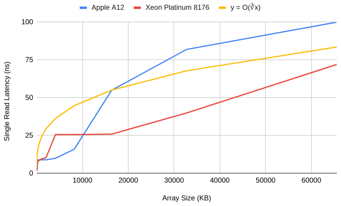
Read latency vs array size for two modern processors. Sources: 1, 2
Notice, however, how poorly the latencies fit the cube-root curve. Memory latency in real processors grows stepwise as a function of each processor’s caches; latency is more or less constant for arrays that fit in the same level of cache, but will quickly jump up once the array is too large and spills into the next level of the memory hierarchy.
If we expand our analysis to even larger datasets–ones that don’t fit in cache–it turns out that speed-of-light effects are insignificant until we reach absurdly large datasets. This is because larger datasets are stored in cheaper and slower storage mediums, and the latency of the medium itself overshadows the speed-of-light effects:
- The fastest and most expensive memory is cache, which is implemented as SRAM. While speed-of-light effects may be significant at this level, a smooth cube-root curve models the latency poorly as detailed above. Besides, it would make more sense to use a square-root rule at this level because caches are part of the processor itself, which must be planar to provide sufficient surface area for cooling.
- The main memory is implemented as DRAM. DRAM’s CAS latency is significant, and maintaining cache coherence (i.e. is the program accessing data that a process from anther core modified?) and CPU-RAM-CPU clock crossings take time too. To put some numbers to this, typical main memory latency is 100+ ns; by then, light could’ve done a 50ft round trip, far more than the physical distance separating RAM and CPU.
- After RAM there’s the computer’s main storage, which is either a spinning hard drive or an SSD. SSDs have far lower latency than spinning disks, but still their latency is in the tens of microseconds–light can travel miles in that time. While the world’s datacenters are approaching a square mile in footprint, they sure aren’t a mile tall.
Disregarding the cube root latency model’s accuracy, the other half of the story is that analyzing algorithms using this model is very awkward. If we assume that memory address has access latency , we’re forcing something continuous–cube root costs–onto something discrete–individual, countable memory addresses–which almost never mixes well. No two memory addresses have the same access cost, and runtimes generally involve sums of cube roots. These sums can generally be simplified by bounding both sides by integrals but that’s a lot of tedious work for a model that isn’t even really accurate.
Zooming out, there are plenty of simplifications besides memory latency that are frequently used in algorithmic analysis. To draw an example from binary search, we assumed that each item of the list occupied space. However, there are only finitely many unique elements representable in space; space is required per element if there are unique elements. Our list therefore either actually takes up space or only has unique items, in which case we could precompute our answer and respond in time.
Such simplifications are not uncommon because a balance needs to be found between the following:
- Simplicity of result and analysis leading to result
- Realism of model
The RAM model is generally good at both, which is why it’s the default. Our cube-root model struggles at both, which is why it and the geometric bound it’s derived from are so obscure. For an overview of memory models that make reasonable sacrifices of 1) for more of 2), check out this MIT 6.851 lecture.